Time-resolved Particle Image Velocimetry: High-speed flow measurement

The Difference Between Standard PIV and Time-Resolved PIV: What Temporal Resolution Changes

The main difference between these two approaches is how they handle time, which directly controls the kind of data you can extract from your experiment. Think of it like signal processing. Imagine trying to capture a moving waveform, like a swirling vortex shedding off a surface, using different sampling rates. If your sampling rate is too low, you under-sample the flow and lose the big picture. 

The Velocity Misconception: Flow Speed vs Flow Timescales

A common mistake when planning an flow measurement experiment is assuming that you need time-resolved PIV for high-velocity flows (like supersonic jets). 
In reality, the choice to go time-resolved is driven by the timescales of the fluid features you want to see, not the absolute speed of the flow. For instance, even in a slow-moving water channel, boundary layer separation bubbles or microfluidic mixing zones can fluctuate rapidly over time. 

 

The Right Tool for the Job

Your choice ultimately simplifies to your data requirements: 

If your research goal is to find statistically stable averages, mean flow fields, and Reynolds Stress Tensors with the highest possible spatial resolution.  

If your research goal is to find the exact time-dependent evolution of fluid structures, continuous pathlines, or frequency-domain data (like PSD).

How Does Time-Resolved PIV Work?

To get true time-resolved data, the system must control laser flashes and camera exposures with microsecond precision. The goal is to perfectly match your laser pulses to your camera's frame rate and the speed of your fluid. 

A standard high-speed PIV setup uses a double-pulse laser running between 1 kHz and 10 kHz or more. Because the laser fires two pulses per cycle, your high-speed camera must run at double the laser's repetition rate to capture each flash on its own image e (e.g., a 1 kHz double pulse laser frequency requires a 2 kHz camera framing rate). 

Depending on how fast your flow is moving and the required time spacing Δt between images, you will use one of two timing methods: 
 

• Correlation: Because the time step between all frames is exactly identical, you can cross-correlate Frame 1 with 2, 2 with 3, 3 with 4, and so on.
• Vector Field Frequency: This gives you a continuous stream of velocity maps at the full frame rate of the camera (e.g., 2,000 vector fields per second from a 2 kHz camera).
• The Reality: This approach is not very common. In most engineering applications, the flow moves too fast for the camera's frame rate, meaning the tracer particles would completely exit the viewing window before the next frame captures them. 
   

• Correlation: You can easily correlate Frame 1 with 2, and Frame 3 with 4. However, you cannot correlate Frame 2 with 3 because the time gap between them is far too wide, and the particles will have travelled completely out of bounds.
• Vector Field Frequency: Because you lose the correlation between the frame pairs, your final vector field frequency drops by half—matching the laser's repetition rate instead of the camera's frame rate (e.g., a 1 kHz laser and 2 kHz camera will yield 1,000 velocity maps per second). 

Key Components and Technical Limitations of a Time-Resolved PIV System

While TR-PIV provides unmatched insights into time-dependent flows, it forces engineers to navigate specific hardware limits and budget trade-offs that do not exist with basic 15 Hz setups. The PIV components below each impose their own ceiling. 

High-Speed PIV Cameras: The Resolution vs. Speed Trade-off	High-Repetition-Rate PIV Lasers: Pulse Energy Power vs Frequency Challenge
Modern high-speed image sensors have incredible light sensitivity, meaning they can easily see light scattering off tiny tracer particles even during microsecond exposures. The true challenge is spatial resolution.	The second major constraint comes from the physics of high-speed solid-state lasers (like diode-pumped Nd:YAG or Nd:YLF systems).
The 2x Rule: To capture a 1 kHz laser rate, the camera has to process 2,000 images every single second. At these speeds, high-speed cameras are typically limited to resolutions of 2 or 4 Megapixels (Mpx). The Resolution Drop: If your experiment requires faster tracking (like 10 kHz or more), the camera sensor must be severely cropped to keep up with the massive flood of data. At ultra-high frame rates, your resolution can quickly plunge to just a few hundred pixels. Financial Overhead: Cameras that can maintain high megapixel resolutions at kilohertz speeds require complex onboard memory and advanced sensors, making them a significant capital investment.	Energy Dilution: Unlike a standard 15 Hz laser that dumps a massive blast of energy into a single pulse, high-speed lasers run on a strict, fixed total power budget. The Trade-off: The more pulses the laser punches out per second, the less energy is available per individual pulse. At 1 kHz, you might have plenty of power to illuminate a wide light sheet ; but at 10 kHz, that energy per pulse drops drastically, forcing you to narrow your light sheet or shrink your field of view to keep the particles bright enough to see.

Synchronizers: Microsecond Timing Control for kHz PIV

At kilohertz repetition rates, the timing hardware stops being a background component and becomes the part that determines whether your data is usable at all. Both equidistant pulsing and frame straddling depend on positioning laser pulses relative to camera frame boundaries with microsecond accuracy and in frame straddling, the two pulses sit on either side of that boundary, so any timing drift destroys the image pair.A dedicated PIV synchronizer generates the trigger pattern for laser and camera, holds the Δt stable across thousands of consecutive cycles, and provides the external trigger inputs you need for phase-locked and transient measurements. It is also the component that lets you couple a PIV system to an external event, such as a rotating shaft or an injection command. 

Tracer Particles and Seeding for High-Speed PIV

Time-resolved PIV places two competing demands on your tracer particles. They must be small enough to faithfully follow the fast fluid features you are trying to resolve, and large enough to scatter sufficient light during a microsecond exposure from a laser pulse whose energy has already been diluted by its own repetition rate.
That balance is why seeding particles and generators deserve attention early in your experimental planning rather than at the end. Seeding density matters just as much: at kHz rates you need a homogeneous particle distribution maintained over the full acquisition period, because a dropout in seeding shows up as a gap in your time series that cannot be recovered by averaging.

Phase-Locked PIV: A Low-Speed Alternative for Rotating Machinery

If you are dealing with strictly repeating, periodic flows, like those inside pumps, turbomachinery, or around cooling fans, there is a clever middle ground called 

How Phase-Locked PIV Triggering Works

This method uses standard, budget-friendly 15 Hz PIV hardware but adds a highly accurate triggering system tied directly to the machine's rotation.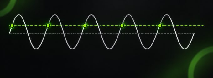 

How Phase-Locked Low-Speed PIV works

A sensor (such as a shaft encoder or optical trigger) tracks the exact angular position of the spinning rotor. The system synchronizer is programmed to only fire the laser and camera when the machine hits a highly specific phase angle during every single rotation (for example, exactly when blade A passes point B). 

 

The results of Phase-Locked Low-Speed PIV works

Instead of random, disconnected snapshots, you collect a sequence of images captured at the exact same phase of the event. Over hundreds or thousands of rotations, you can stack these phase-averaged frames together to build a high-resolution, 3D reconstruction of the flow features relative to the moving blade and by combining this with a stereo PIV setup, all three velocity components.

 

advantages and limitations of phase-locked PIV

Advantages	Limitations
Uses standard PIV hardware, keeping system costs low.	Only works for strictly periodic or rotating flows.
Delivers incredible spatial resolution (often better than high-speed TR-PIV systems).	Huge data acquisition overhead; you must take thousands of measurements to reconstruct a full cycle.
Perfect for isolating and stabilizing stationary statistical flow patterns.	Completely blind to cycle-to-cycle or sudden transient variations. It cannot show you if one vortex sheds differently than the last.

Typical Applications of Time-Resolved and Phase-Locked PIV

Particle Image Velocimetry is an essential troubleshooting and diagnostic tool across a wide range of applications and industries

A New Frontier: Event-Based PIV

While high-speed cameras and pulsed lasers are the traditional choices for time-resolved PIV, a new alternative has arrived: Event-Based PIV. This technique uses neuromorphic, "event-based" cameras that completely flip how visual data is recorded. Our validation study of the flow convergence method shows how PIV benchmarks established clinical measurement approaches in pulsatile in vitro environments.

High-Speed Flow Measurement Without a Pulsed Laser

Standard cameras take a full picture of the entire scene at fixed intervals, processing every pixel whether it changed or not. Event-based sensors feature pixels that operate completely independently and asynchronously from one another. 

How Event-Based Cameras Work: Pixel-Level Independence

Instead of waiting for a camera shutter frame, an event-based pixel only reports data the exact microsecond it notices a change in light intensity. If its view stays completely constant, the pixel remains totally silent. 

• Imagine a fluid field filled with reflective tracking particles. As a particle moves, it crosses into a pixel's view, causing a quick spike in brightness. The pixel instantly fires an "event" containing three simple values: its X-coordinate, its Y-coordinate, and a precise microsecond timestamp. As the particle moves past, the pixel sees the light drop and fires a second event. 

Limitations of Event-Based PIV

The main limitation of current event-based technology is spatial resolution, which usually tops out around 1 Mpx. However, when you consider that a traditional high-speed camera must be cropped and lose resolution to hit 10 kHz, maintaining a full 1 Mpx at 10 kHz makes event-based tracking a highly competitive option.

The Advantages of Event-Based PIV

Because the camera only records active changes, it completely cuts out the massive data overhead that slows down traditional high-speed setups. This brings massive operational benefits: 

• Continuous Light Sources: Since the pixels respond to continuous movement, you do not need a pulsed laser. Event-Based PIV works perfectly with continuous-wave (CW) lasers or simple, high-power LEDs.
• Ultra-High Speed: The sensor can easily track particle speeds that match sampling rates of 10 kHz or more.
• Instant, Live Data Analysis: Because the data stream is incredibly lightweight (only transmitting coordinates that are moving, rather than megabytes of static background pictures), processing is lightning-fast. The data can be calculated instantly, giving you a live velocity field output while your experiment is running.
• Drastically Lower Cost: By removing the need for specialized high-speed camera and pulsed lasers, an Event-Based PIV system costs a fraction of a traditional TR-PIV setup.